50 SQL Interview Questions and Answers With Examples

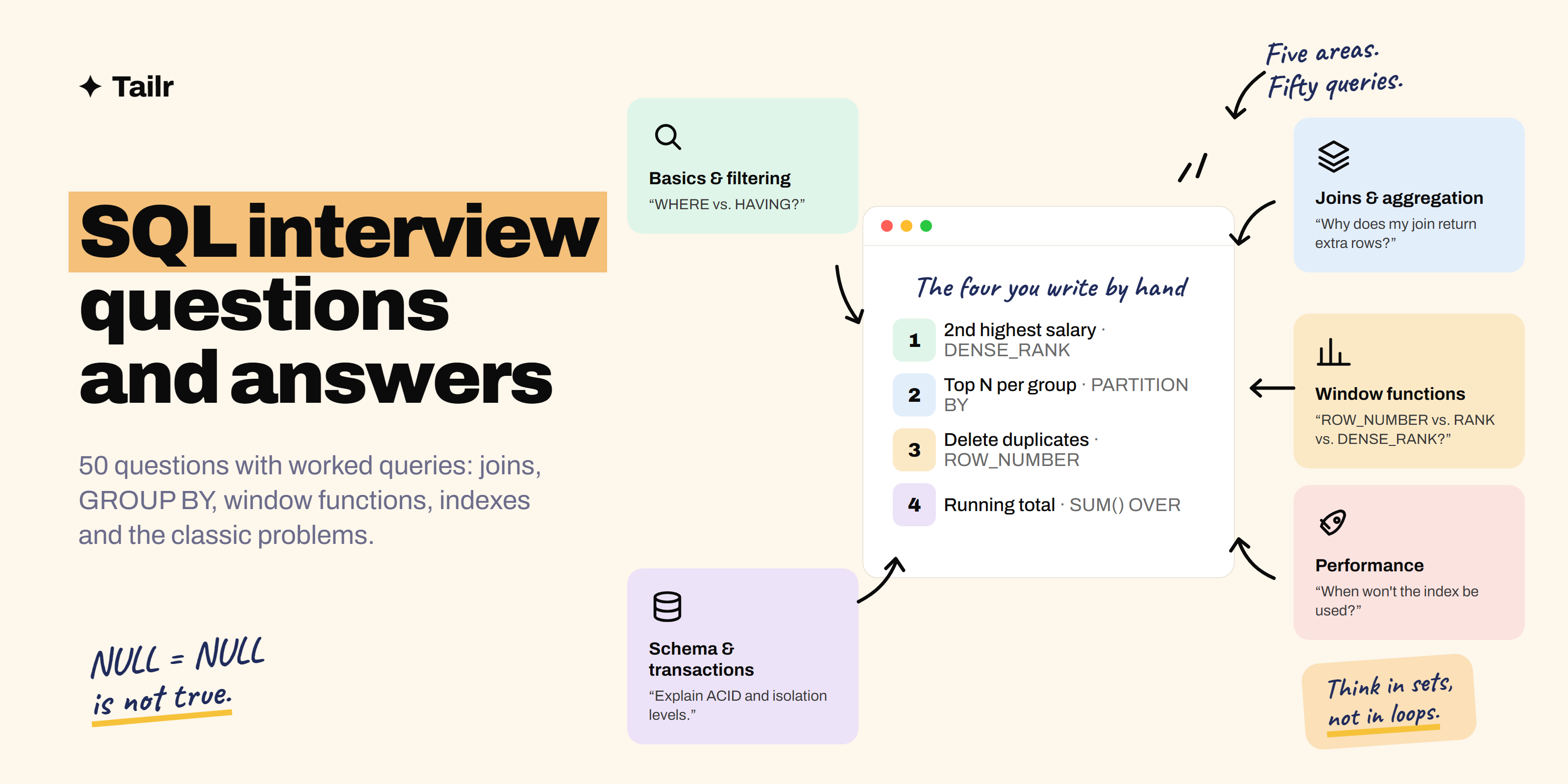
SQL comes up in more interviews than any other technical skill: analyst, backend, data engineering, QA, product, and increasingly product management and marketing ops. The questions repeat. This page has the 50 that come up most, grouped from basics to optimisation, each with a worked answer and a query you can write on a whiteboard. Where a fresher answer and an experienced answer differ, both are given.

The short answer: SQL interviews cover five areas:

• Basics and filtering: WHERE vs HAVING, DISTINCT, NULL handling.
• Joins and aggregation: every join type, GROUP BY pitfalls, UNION vs UNION ALL.
• Window functions and the classic problems: second highest salary, duplicates, top-N per group, running totals, consecutive days.
• Schema and integrity: keys, constraints, normalisation, ACID, isolation levels.
• Performance: indexes, EXPLAIN, why an index isn’t used, N+1.

Learn window functions properly and practise the ten classic problems by hand, and you’ll handle most of what’s below.

The examples use a small schema of three tables, employees, departments and orders; the CREATE TABLE statements are just below so you can run everything yourself. Syntax is standard SQL; dialect differences are noted where they matter.

The sample schema used below

Most of the answers use these three tables, so you can run them yourself. Syntax is Postgres unless a dialect difference is worth knowing, in which case it’s called out.

CREATE TABLE departments (
  id    INT PRIMARY KEY,
  name  TEXT NOT NULL
);

CREATE TABLE employees (
  id             INT PRIMARY KEY,
  name           TEXT NOT NULL,
  department_id  INT REFERENCES departments(id),
  manager_id     INT REFERENCES employees(id),
  salary         NUMERIC(10, 2),
  hired_on       DATE
);

CREATE TABLE orders (
  id           INT PRIMARY KEY,
  customer_id  INT NOT NULL,
  ordered_on   DATE NOT NULL,
  amount       NUMERIC(10, 2) NOT NULL
);

Basics and filtering

1. What’s the difference between WHERE and HAVING?

WHERE filters rows before grouping; HAVING filters groups after aggregation. Aggregates can’t go in WHERE because the groups don’t exist yet.

SELECT customer_id, COUNT(*) AS orders
FROM orders
WHERE ordered_on >= '2026-01-01'   -- filters individual rows first
GROUP BY customer_id
HAVING COUNT(*) > 5;               -- then filters the groups

A useful way to say it: WHERE decides which rows get counted; HAVING decides which counts get shown.

2. In what order does SQL evaluate a query?

You write it in one order and the database runs it in another:

Step	Clause	What it does
1	FROM, JOIN	Builds the working set of rows
2	WHERE	Filters rows
3	GROUP BY	Collapses rows into groups
4	HAVING	Filters groups
5	SELECT	Computes the output columns (and aliases)
6	DISTINCT	Removes duplicate output rows
7	ORDER BY	Sorts the result
8	LIMIT / OFFSET	Trims it

This explains two things people trip over. First, you can’t use a SELECT alias in WHERE, because WHERE runs before SELECT:

SELECT salary * 12 AS annual
FROM employees
WHERE annual > 100000;      -- error in most databases: "annual" doesn't exist yet

-- fix: repeat the expression, or wrap it in a subquery or CTE
SELECT salary * 12 AS annual
FROM employees
WHERE salary * 12 > 100000;

Second, you can use that alias in ORDER BY, because ORDER BY runs after SELECT.

3. What does DISTINCT do, and what’s the cost?

Removes duplicate rows from the result. It requires a sort or hash over the whole result set, so on large results it’s expensive. If you find yourself adding DISTINCT to fix duplicated rows from a join, the join is probably wrong; fix the join instead (see question 14).

4. How does SQL treat NULL?

NULL is unknown, not zero and not empty. Everything that follows comes from that one idea:

• NULL = NULL is not true (it’s unknown), so you must write IS NULL, never = NULL.
• Any arithmetic or comparison with NULL yields NULL: 5 + NULL is NULL, 'a' = NULL is unknown.
• Aggregates ignore NULLs: COUNT(col) skips them, AVG(col) averages only the non-null values. COUNT(*) counts every row.
• COALESCE(col, 0) substitutes a default; NULLIF(a, b) returns NULL when a = b, which is how you avoid divide-by-zero.

The classic bug is NOT IN with a NULL in the list:

-- returns NO rows if any department_id is NULL in departments
SELECT * FROM employees
WHERE department_id NOT IN (SELECT id FROM departments);

Why: x NOT IN (1, 2, NULL) expands to x <> 1 AND x <> 2 AND x <> NULL. The last part is unknown, so the whole condition is unknown, so no row passes. Use NOT EXISTS instead:

SELECT * FROM employees e
WHERE NOT EXISTS (SELECT 1 FROM departments d WHERE d.id = e.department_id);

5. What’s the difference between COUNT(*), COUNT(col) and COUNT(DISTINCT col)?

COUNT(*) counts rows. COUNT(col) counts rows where col is not NULL. COUNT(DISTINCT col) counts unique non-NULL values. With this data:

id	department_id
1	10
2	10
3	NULL
4	20

COUNT(*) = 4, COUNT(department_id) = 3, COUNT(DISTINCT department_id) = 2.

6. What’s the difference between DELETE, TRUNCATE and DROP?

	DELETE	TRUNCATE	DROP
Removes	Rows (optionally with WHERE)	All rows	The table itself
Speed	Row by row	Deallocates pages; fast	Immediate
Logging	Every row	Minimal	Minimal
Triggers	Fire	Don’t fire	N/A
Identity reset	No	Usually yes	N/A
Rollback	Yes	Depends on database (yes in Postgres, no in MySQL)	Depends

If someone asks “how do you empty a big table quickly”, the answer is TRUNCATE; if they ask “how do you remove last year’s rows”, it’s DELETE with a WHERE, possibly in batches.

7. What’s the difference between UNION and UNION ALL?

UNION removes duplicates (and sorts or hashes to do it); UNION ALL keeps everything and is faster.

SELECT 'a' AS x UNION     SELECT 'a';   -- one row
SELECT 'a' AS x UNION ALL SELECT 'a';   -- two rows

Use UNION ALL unless you specifically need de-duplication. Saying “I default to UNION ALL and switch only when I’ve thought about duplicates” is the answer interviewers want.

8. What’s the difference between IN and EXISTS?

Both filter by a subquery, and on modern optimisers they usually produce the same plan. The differences that matter:

-- IN: the subquery produces a list of values
SELECT * FROM employees
WHERE department_id IN (SELECT id FROM departments WHERE name = 'Sales');

-- EXISTS: the subquery is a yes/no check per outer row
SELECT * FROM employees e
WHERE EXISTS (SELECT 1 FROM departments d
              WHERE d.id = e.department_id AND d.name = 'Sales');

EXISTS stops at the first match and is safe with NULLs; IN is easier to read for a simple list. For the negative case, always prefer NOT EXISTS over NOT IN because of the NULL problem in question 4.

9. What does LIMIT / TOP / FETCH do, and how do you paginate?

Restricts the number of rows returned. The keyword varies by dialect:

SELECT * FROM orders ORDER BY id LIMIT 10 OFFSET 20;          -- Postgres, MySQL, SQLite
SELECT TOP 10 * FROM orders ORDER BY id;                      -- SQL Server
SELECT * FROM orders ORDER BY id OFFSET 20 ROWS FETCH NEXT 10 ROWS ONLY;  -- standard, SQL Server, Oracle

Offset pagination gets slow on deep pages because the database still has to read and discard the first 20 (or 20,000) rows. Keyset pagination fixes it by remembering the last row you saw:

-- page 1
SELECT * FROM orders ORDER BY id LIMIT 10;
-- page 2: pass the last id from page 1
SELECT * FROM orders WHERE id > 1043 ORDER BY id LIMIT 10;

It’s O(page size) regardless of depth, and it doesn’t skip or duplicate rows when new data arrives between pages. The cost: you can’t jump to page 50 directly.

10. What’s the difference between CHAR and VARCHAR?

CHAR is fixed-length and padded with spaces; VARCHAR is variable-length and stores only what you insert. CHAR(5) storing 'ab' holds 'ab '. Use VARCHAR unless every value is the same length (two-letter country codes, say), and in Postgres just use TEXT.

Joins and aggregation

11. Explain every join type.

Use two tiny tables to make it concrete:

employees

id	name	department_id
1	Ana	10
2	Ben	20
3	Cal	NULL

departments

id	name
10	Sales
30	Legal

• INNER JOIN: only rows with a match on both sides. Result: Ana / Sales. One row.
• LEFT JOIN: every employee, with department where it matches and NULL where it doesn’t. Result: Ana / Sales, Ben / NULL, Cal / NULL. Three rows.
• RIGHT JOIN: every department, with employee where it matches. Result: Ana / Sales, NULL / Legal. Rarely used; rewrite as a LEFT JOIN with the tables swapped.
• FULL OUTER JOIN: everything from both sides. Result: Ana / Sales, Ben / NULL, Cal / NULL, NULL / Legal. Four rows. MySQL doesn’t support it; emulate with a LEFT JOIN UNION a RIGHT JOIN.
• CROSS JOIN: every combination, 3 × 2 = 6 rows. Useful for generating date ranges or test data.
• SELF JOIN: a table joined to itself, for hierarchies like employee and manager (question 13).

If you can draw these four result sets on a whiteboard from memory, you’ve answered the question.

12. Write a query to find employees who have no department.

SELECT e.*
FROM employees e
LEFT JOIN departments d ON d.id = e.department_id
WHERE d.id IS NULL;

The LEFT JOIN plus IS NULL on the right side is the anti-join pattern. NOT EXISTS (question 4) is the alternative and reads more clearly to many people; either is fine.

13. Write a query to list each employee with their manager’s name.

SELECT e.name AS employee, m.name AS manager
FROM employees e
LEFT JOIN employees m ON m.id = e.manager_id;

LEFT, not INNER, so the CEO with no manager still appears (with a NULL manager). Aliasing the same table twice (e and m) is the whole trick of a self join.

14. Why does my join return more rows than I expected?

Because the join key isn’t unique on one side: one row on the left matches several on the right, and the result multiplies. Here’s how to prove it and fix it:

-- 1. find the offending keys
SELECT department_id, COUNT(*)
FROM employees
GROUP BY department_id
HAVING COUNT(*) > 1;

-- 2. fix: aggregate the many side BEFORE joining
SELECT d.name, e.headcount
FROM departments d
JOIN (
  SELECT department_id, COUNT(*) AS headcount
  FROM employees
  GROUP BY department_id
) e ON e.department_id = d.id;

Adding DISTINCT to the outer query hides the problem and often gives wrong totals. Pre-aggregating the many side, or fixing the join condition, solves it.

15. What’s the difference between a join condition in ON and in WHERE?

For an INNER JOIN, none. For a LEFT JOIN it changes the meaning entirely:

-- keeps every employee; department name is NULL unless it's Sales
SELECT e.name, d.name
FROM employees e
LEFT JOIN departments d ON d.id = e.department_id AND d.name = 'Sales';

-- silently becomes an INNER JOIN: the WHERE throws away the NULL rows
SELECT e.name, d.name
FROM employees e
LEFT JOIN departments d ON d.id = e.department_id
WHERE d.name = 'Sales';

Rule: conditions on the right table of a LEFT JOIN belong in ON. Conditions on the left table can go in WHERE.

16. Write a query for average salary by department, only departments with more than three employees, highest first.

SELECT d.name, AVG(e.salary) AS avg_salary
FROM employees e
JOIN departments d ON d.id = e.department_id
GROUP BY d.name
HAVING COUNT(*) > 3
ORDER BY avg_salary DESC;

Walk through it in evaluation order (question 2): join, group by department, keep groups with more than three rows, compute the average, sort.

17. Why does “column must appear in GROUP BY” happen?

Because every column in SELECT must be either aggregated or in the GROUP BY; otherwise the database doesn’t know which row’s value to show.

-- error: which employee's "name" should appear for department 10?
SELECT department_id, name, AVG(salary)
FROM employees
GROUP BY department_id;

Three ways out, depending on what you actually meant:

-- a) you wanted one row per (department, name)
SELECT department_id, name, AVG(salary) FROM employees GROUP BY department_id, name;

-- b) you wanted any one name, and don't care which
SELECT department_id, MAX(name), AVG(salary) FROM employees GROUP BY department_id;

-- c) you wanted every employee alongside their department average
SELECT department_id, name, AVG(salary) OVER (PARTITION BY department_id) FROM employees;

MySQL historically allowed the original query and picked an arbitrary row, which caused silent bugs; since 5.7 it rejects it by default.

18. What’s the difference between GROUP BY and a window function?

GROUP BY collapses rows into one per group. A window function computes over the group but keeps every row. If you need the department average next to each employee’s salary, that’s a window function:

SELECT name, salary,
       AVG(salary) OVER (PARTITION BY department_id) AS dept_avg,
       salary - AVG(salary) OVER (PARTITION BY department_id) AS diff_from_avg
FROM employees;

name	salary	dept_avg	diff_from_avg
Ana	90000	80000	10000
Ben	70000	80000	-10000

Rule of thumb: if the question says “per department, how many”, it’s GROUP BY. If it says “for each employee, compared with their department”, it’s a window.

19. What is a CTE, and when would you use one over a subquery?

A Common Table Expression (WITH name AS (...)) is a named subquery. Compare the same query both ways:

-- nested subquery
SELECT name FROM (
  SELECT name, salary, AVG(salary) OVER () AS avg_all FROM employees
) t WHERE salary > avg_all;

-- CTE: reads top to bottom
WITH with_avg AS (
  SELECT name, salary, AVG(salary) OVER () AS avg_all FROM employees
)
SELECT name FROM with_avg WHERE salary > avg_all;

Use a CTE when a query has several steps, when the same subquery is reused, and for recursion. Performance is usually identical; in Postgres before version 12, CTEs were an optimisation fence (always materialised), which is why some older advice avoids them.

20. Write a recursive CTE to list all reports under a given manager.

WITH RECURSIVE reports AS (
  -- anchor: start with the manager
  SELECT id, name, manager_id, 0 AS depth
  FROM employees WHERE id = 42
  UNION ALL
  -- recursive step: add everyone whose manager is already in the result
  SELECT e.id, e.name, e.manager_id, r.depth + 1
  FROM employees e
  JOIN reports r ON e.manager_id = r.id
)
SELECT * FROM reports WHERE id <> 42 ORDER BY depth, name;

How it runs, step by step:

1. The anchor query runs once and produces the manager (depth 0).
2. The recursive step runs against the rows from step 1 and finds their direct reports (depth 1).
3. It runs again against the depth-1 rows and finds depth 2, and so on.
4. It stops when a step produces no new rows.

The depth column isn’t required, but it’s a good habit: it lets you order the output and, with WHERE r.depth < 20, protect yourself if the data contains a cycle. SQL Server and Oracle omit the RECURSIVE keyword; the shape is the same.

Window functions and the classic problems

21. Explain ROW_NUMBER, RANK and DENSE_RANK.

All three number rows within a partition in an order; they differ only in how they treat ties.

SELECT name, salary,
       ROW_NUMBER() OVER (ORDER BY salary DESC) AS row_num,
       RANK()       OVER (ORDER BY salary DESC) AS rnk,
       DENSE_RANK() OVER (ORDER BY salary DESC) AS dense
FROM employees;

name	salary	row_num	rnk	dense
Ana	100	1	1	1
Ben	100	2	1	1
Cal	90	3	3	2

ROW_NUMBER breaks ties arbitrarily (add a tiebreaker to the ORDER BY if you need it deterministic). RANK skips numbers after a tie. DENSE_RANK doesn’t. Pick based on what “second highest” should mean when two people share the top spot.

22. Find the second highest salary.

Fresher answer (subquery):

SELECT MAX(salary) FROM employees
WHERE salary < (SELECT MAX(salary) FROM employees);

Experienced answer (window, generalises to nth):

SELECT salary FROM (
  SELECT salary, DENSE_RANK() OVER (ORDER BY salary DESC) AS rnk
  FROM employees
) t
WHERE rnk = 2;

Mention that DENSE_RANK handles ties (two people on the top salary still gives a real second), that the window version returns nothing rather than NULL when there’s only one salary, and that SELECT DISTINCT salary ORDER BY salary DESC LIMIT 1 OFFSET 1 is a third option.

23. Find the top three earners in each department.

SELECT * FROM (
  SELECT e.*,
         DENSE_RANK() OVER (PARTITION BY department_id ORDER BY salary DESC) AS rnk
  FROM employees e
) t
WHERE rnk <= 3;

This is the “top N per group” pattern; it comes up in some form in most interviews. The subquery is needed because you can’t filter on a window function in the same SELECT’s WHERE (question 2 again: WHERE runs before SELECT).

24. Find duplicate rows.

SELECT name, department_id, COUNT(*)
FROM employees
GROUP BY name, department_id
HAVING COUNT(*) > 1;

25. Delete duplicates, keeping the row with the lowest id.

WITH ranked AS (
  SELECT id,
         ROW_NUMBER() OVER (PARTITION BY name, department_id ORDER BY id) AS rn
  FROM employees
)
DELETE FROM employees WHERE id IN (SELECT id FROM ranked WHERE rn > 1);

Say you’d run the SELECT first to see what would be deleted, wrap it in a transaction, and that MySQL needs a slightly different form (join the derived table in the DELETE) because it can’t delete from a table it’s reading in the same statement.

26. Compute a running total of order amounts by date.

SELECT ordered_on, amount,
       SUM(amount) OVER (ORDER BY ordered_on, id) AS running_total
FROM orders;

ordered_on	amount	running_total
2026-03-01	50	50
2026-03-01	20	70
2026-03-02	30	100

Include a tiebreaker (id) in the ORDER BY so the total is deterministic when two orders share a date. Add PARTITION BY customer_id for a running total per customer.

27. Compare each order with the previous order from the same customer.

SELECT customer_id, ordered_on, amount,
       LAG(amount) OVER (PARTITION BY customer_id ORDER BY ordered_on) AS prev_amount,
       amount - LAG(amount) OVER (PARTITION BY customer_id ORDER BY ordered_on) AS change
FROM orders;

LEAD does the same for the next row. The first row in each partition gets NULL for prev_amount; pass a default as the third argument (LAG(amount, 1, 0)) if you’d rather have zero. This is how you compute day-over-day change without a self-join.

28. Find customers who ordered on three or more consecutive days.

The gaps-and-islands pattern: subtract a row number from the date so consecutive days share a group key. Seeing it on a table makes it click:

ordered_on	row_number	date − row_number
Mar 1	1	Feb 28
Mar 2	2	Feb 28
Mar 3	3	Feb 28
Mar 7	4	Mar 3
Mar 8	5	Mar 3

Consecutive dates increase by one, and so does the row number, so the difference stays constant within a run and jumps at every gap. Group by that difference and count.

WITH d AS (
  SELECT DISTINCT customer_id, ordered_on FROM orders
), g AS (
  SELECT customer_id, ordered_on,
         ordered_on - ROW_NUMBER() OVER (PARTITION BY customer_id ORDER BY ordered_on) * INTERVAL '1 day' AS grp
  FROM d
)
SELECT customer_id, MIN(ordered_on) AS start_day, COUNT(*) AS days
FROM g
GROUP BY customer_id, grp
HAVING COUNT(*) >= 3;

The DISTINCT in the first CTE matters: two orders on the same day would otherwise get two row numbers and break the arithmetic. Date arithmetic differs by dialect (DATE_SUB in MySQL, DATEADD in SQL Server); say so rather than getting it exactly right on a whiteboard.

29. Find the month-over-month percentage change in revenue.

WITH m AS (
  SELECT DATE_TRUNC('month', ordered_on) AS month, SUM(amount) AS revenue
  FROM orders
  GROUP BY 1
)
SELECT month, revenue,
       LAG(revenue) OVER (ORDER BY month) AS prev_revenue,
       100.0 * (revenue - LAG(revenue) OVER (ORDER BY month))
             / NULLIF(LAG(revenue) OVER (ORDER BY month), 0) AS pct_change
FROM m;

Two details interviewers look for: the 100.0 (not 100) forces decimal division in databases that would otherwise do integer maths, and NULLIF(..., 0) stops a zero-revenue month from raising a divide-by-zero error. Months with no orders at all won’t appear; if that matters, generate a month series and LEFT JOIN to it.

30. Pivot rows to columns: revenue per month as one row per year.

Standard SQL uses conditional aggregation:

SELECT EXTRACT(YEAR FROM ordered_on) AS yr,
       SUM(CASE WHEN EXTRACT(MONTH FROM ordered_on) = 1 THEN amount END) AS jan,
       SUM(CASE WHEN EXTRACT(MONTH FROM ordered_on) = 2 THEN amount END) AS feb,
       SUM(CASE WHEN EXTRACT(MONTH FROM ordered_on) = 3 THEN amount END) AS mar
FROM orders
GROUP BY 1
ORDER BY 1;

The CASE returns NULL for rows that aren’t that month, and SUM ignores NULLs, so each column only adds up its own month. SQL Server and Oracle have a PIVOT keyword; Postgres has crosstab and FILTER (WHERE ...). The CASE version works everywhere, and it’s the one to write in an interview.

31. Find employees hired in the last 90 days who earn above their department average.

SELECT name, salary FROM (
  SELECT e.*, AVG(salary) OVER (PARTITION BY department_id) AS dept_avg
  FROM employees e
) t
WHERE hired_on >= CURRENT_DATE - INTERVAL '90 days' AND salary > dept_avg;

Note the average is computed over all employees in the department, not just recent hires, because the window is applied before the WHERE filters the outer query. If the interviewer wanted the average of recent hires only, the filter would move inside the subquery. Ask which they mean.

32. Find the median salary.

No standard MEDIAN function exists everywhere. In Postgres it’s one line:

SELECT PERCENTILE_CONT(0.5) WITHIN GROUP (ORDER BY salary) FROM employees;

Portable version: number the rows from both ends and average the middle one or two.

WITH r AS (
  SELECT salary,
         ROW_NUMBER() OVER (ORDER BY salary) AS asc_n,
         ROW_NUMBER() OVER (ORDER BY salary DESC) AS desc_n
  FROM employees
)
SELECT AVG(salary) FROM r WHERE asc_n IN (desc_n, desc_n - 1, desc_n + 1);

Why the condition works: with an odd count (say 5), the middle row has asc_n = desc_n = 3. With an even count (say 6), the two middle rows have (3, 4) and (4, 3), so each is within one of the other, and AVG takes their mean. Every other row is further apart than that.

Schema, keys and transactions

33. What’s the difference between a primary key and a unique key?

Both enforce uniqueness. A table has one primary key, which can’t be NULL and is usually the clustered index; it can have many unique constraints, which allow NULL (one NULL in SQL Server, any number in Postgres and MySQL, because NULLs aren’t equal to each other). Foreign keys can reference either.

CREATE TABLE users (
  id     INT PRIMARY KEY,           -- one per table, NOT NULL implied
  email  TEXT UNIQUE,               -- as many as you need
  handle TEXT UNIQUE
);

34. What is a foreign key, and what happens on delete?

A column that must match a key in another table, which stops you creating an order for a customer that doesn’t exist. What happens when the parent row is deleted is up to you:

CREATE TABLE orders (
  id           INT PRIMARY KEY,
  customer_id  INT REFERENCES customers(id) ON DELETE RESTRICT   -- block the delete (default)
  -- ... ON DELETE CASCADE    -- delete this customer's orders too
  -- ... ON DELETE SET NULL   -- keep the orders, orphan them
);

Know which one your schema uses. CASCADE on the wrong table (say, deleting a department cascades to its employees) removes a lot of data very quickly.

35. Explain normalisation and the first three normal forms.

Start from a table that breaks all three and fix it one form at a time.

Unnormalised:

order_id	customer	customer_city	products
1	Ana	Leeds	pen, notebook

• 1NF: atomic values, no repeating groups. Split products into one row per product (an order_items table).
• 2NF: every non-key column depends on the whole primary key. In order_items with key (order_id, product_id), a column like product_name depends only on product_id, so it moves to a products table. This only bites with composite keys.
• 3NF: no non-key column depends on another non-key column. customer_city depends on customer, not on order_id, so customers get their own table.

The practical version: don’t store the same fact in two places, because one copy will be updated and the other won’t. Denormalise deliberately for read performance, and know you did.

36. What is ACID?

Atomicity (all or nothing), Consistency (constraints hold before and after), Isolation (concurrent transactions don’t see each other’s half-done work), Durability (committed means saved, even if the power goes). The example everyone uses: moving money between accounts.

BEGIN;
UPDATE accounts SET balance = balance - 100 WHERE id = 1;
UPDATE accounts SET balance = balance + 100 WHERE id = 2;
COMMIT;   -- or ROLLBACK, and neither update happens

Interviewers usually follow with question 37.

37. What are isolation levels, and what problems do they prevent?

Level	Dirty read	Non-repeatable read	Phantom read	Default in
Read Uncommitted	Possible	Possible	Possible	(rarely used)
Read Committed	Prevented	Possible	Possible	Postgres, SQL Server, Oracle
Repeatable Read	Prevented	Prevented	Possible (prevented in Postgres)	MySQL InnoDB
Serializable	Prevented	Prevented	Prevented

The three problems, in plain words:

• Dirty read: you see another transaction’s uncommitted change, and it then rolls back.
• Non-repeatable read: you read a row, someone commits an update, you read the same row again and it’s different.
• Phantom read: you run WHERE amount > 100, someone inserts a matching row, you run it again and get an extra row.

Higher isolation means more locking or more retries on conflict, so the default is usually right unless you’re doing something like “read a balance, then update it based on what you read”, which needs Serializable or an explicit lock (SELECT ... FOR UPDATE).

38. What is a deadlock, and how do you avoid one?

Two transactions each holding a lock the other needs, so neither can proceed:

Time	Transaction A	Transaction B
1	UPDATE accounts WHERE id = 1 (locks row 1)
2		UPDATE accounts WHERE id = 2 (locks row 2)
3	UPDATE accounts WHERE id = 2 (waits for B)
4		UPDATE accounts WHERE id = 1 (waits for A) → deadlock

The database detects the cycle and kills one transaction, which the application must retry. Avoid it by:

1. Acquiring locks in a consistent order (always update the lower id first).
2. Keeping transactions short; never hold one open across user input or a network call.
3. Updating in one statement where possible (UPDATE ... WHERE id IN (1, 2)).
4. Retrying on deadlock errors in application code, because you can’t prevent them entirely.

39. What’s the difference between a clustered and a non-clustered index?

A clustered index defines the physical order of the table’s rows on disk; there’s one per table (the primary key by default in SQL Server and MySQL InnoDB). Non-clustered indexes are separate structures that point at rows, and you can have many. A lookup through a non-clustered index finds the pointer, then fetches the row; a lookup through the clustered index finds the row directly. Postgres has no clustered index in the same sense (CLUSTER reorders once but doesn’t maintain it); all its indexes are secondary.

40. What’s a view, and what’s a materialised view?

A view is a saved query that runs when you select from it: no storage, always current. A materialised view stores the result and must be refreshed: fast to read, possibly stale.

CREATE VIEW active_employees AS
  SELECT * FROM employees WHERE left_on IS NULL;

CREATE MATERIALIZED VIEW monthly_revenue AS
  SELECT DATE_TRUNC('month', ordered_on) AS month, SUM(amount) AS revenue
  FROM orders GROUP BY 1;

REFRESH MATERIALIZED VIEW monthly_revenue;   -- on a schedule, or after loads

Use views for reuse and access control; use materialised views for expensive aggregations that are read often and change rarely.

Performance

41. What is an index, and how does it work?

A separate structure (usually a B-tree) that maps column values to row locations, so the database can find rows without scanning the table. Think of the index at the back of a book: sorted, so you can binary-search it, with a page number for each entry.

CREATE INDEX idx_employees_department ON employees (department_id);

Indexes speed up reads on the indexed columns and slow down writes, because every insert, update and delete has to maintain them. A table with ten indexes is slow to write to. The skill is choosing the few that serve the queries you actually run.

42. When will the database not use an index?

• The query wraps the column in a function: WHERE YEAR(hired_on) = 2026.
• A leading wildcard: WHERE name LIKE '%son'.
• Implicit type conversion: comparing a VARCHAR column to a number.
• The query touches most of the table, so a scan is cheaper anyway.
• A composite index (a, b) and the query filters only on b.
• Statistics are stale, so the planner misjudges the cost.

The first one is the most common, and the fix is to rewrite the condition as a range on the raw column:

-- can't use the index on hired_on
WHERE YEAR(hired_on) = 2026

-- can
WHERE hired_on >= '2026-01-01' AND hired_on < '2027-01-01'

43. How do you read an EXPLAIN plan?

Run EXPLAIN ANALYZE (Postgres) or EXPLAIN (MySQL) in front of the query and read the tree from the innermost node outward. Here’s a Postgres plan for a query that’s missing an index:

Hash Join  (cost=1.09..3521.40 rows=48000 width=40) (actual time=0.05..41.2 rows=48000 loops=1)
  Hash Cond: (e.department_id = d.id)
  ->  Seq Scan on employees e  (cost=0.00..2900.00 rows=200000 width=32) (actual ...)
        Filter: (salary > 50000)
        Rows Removed by Filter: 152000
  ->  Hash  (cost=1.04..1.04 rows=4 width=12)
        ->  Seq Scan on departments d  ...

What to look for, in order:

1. Full scans on big tables. Seq Scan in Postgres, type: ALL in MySQL. Here the 200,000-row employees scan with 152,000 rows removed by the filter is the problem; an index on salary would turn it into an Index Scan.
2. Estimated vs. actual rows. A big gap (rows=100 estimated, rows=90000 actual) means stale statistics; run ANALYZE.
3. Join method. A Nested Loop over a large outer table is a warning; Hash Join and Merge Join scale better.
4. Sorts and spills. Sort Method: external merge Disk means the sort didn’t fit in memory.

Start with the most expensive node and work back; fixing it usually changes the whole plan.

44. What is a composite index, and does column order matter?

An index on more than one column. Order matters because the index is sorted by the first column, then by the second within it, like a phone book sorted by surname then first name.

CREATE INDEX idx_dept_salary ON employees (department_id, salary);

This index serves WHERE department_id = 3 and WHERE department_id = 3 AND salary > 50000, but not WHERE salary > 50000 alone, just as a phone book doesn’t help you find everyone called “Sam”. Rule: put equality columns first, then the range column, then columns you only need for sorting or covering.

45. What is a covering index?

An index that contains every column the query needs, so the database answers from the index without touching the table at all (an “index-only scan”).

-- the query
SELECT department_id, salary FROM employees WHERE department_id = 3;

-- an index that covers it
CREATE INDEX idx_dept_cover ON employees (department_id) INCLUDE (salary);   -- Postgres, SQL Server
CREATE INDEX idx_dept_cover ON employees (department_id, salary);            -- MySQL, Oracle

It’s the cheapest big win for a hot read query, at the cost of a larger index.

46. What is the N+1 query problem?

An application fetches a list (one query), then runs one query per item to fetch related data (N more). For 100 departments that’s 101 round-trips:

SELECT id, name FROM departments;                        -- 1 query
SELECT * FROM employees WHERE department_id = 1;         -- then 100 of these
SELECT * FROM employees WHERE department_id = 2;
...

Fix with a join, or one batched query:

SELECT * FROM employees WHERE department_id IN (1, 2, 3, ...);   -- 1 query

It’s usually an ORM issue (lazy loading in a loop), and every ORM has an “eager load” option for exactly this. The interviewer wants to hear that you’d spot it in the query log: the same statement repeating with different parameters is the giveaway.

47. How would you speed up a slow query?

In order, stopping when it’s fast enough:

1. Look at the plan (question 43) and find the expensive node.
2. Add or fix an index for the WHERE and JOIN columns.
3. Remove functions and implicit casts on indexed columns (question 42).
4. Select only the columns you need, so a covering index becomes possible.
5. Check the join isn’t multiplying rows (question 14).
6. Replace correlated subqueries with joins or window functions.
7. Pre-aggregate with a materialised view if the query is run often and the data changes rarely.
8. Only then consider denormalising or caching in the application.

Interviewers like hearing “measure first” and a specific story about a query you actually fixed.

48. What is a query hint, and why avoid them?

A directive that forces the optimiser’s choice: a specific index, a join order, a join method (/*+ INDEX(...) */ in Oracle, WITH (INDEX(...)) in SQL Server, FORCE INDEX in MySQL). They fix today’s problem and break next year’s when data distribution changes and the forced plan is no longer the good one. Fix statistics or indexes instead; use hints as a last resort and comment why they’re there.

Scenarios

49. A report’s numbers don’t match the source system. How do you find the difference?

Reconcile from the top down:

1. Totals first. Compare row count and total amount for the whole period. If those match, the problem is in a breakdown, not the data.
2. Narrow by time. Compare per day. The mismatch usually clusters in one day or at a boundary.
3. Narrow by dimension. Compare per customer, per product, per region for that day.
4. Diff the rows. Once you’re down to a small set, find the exact rows on one side but not the other:

SELECT id, amount FROM report_orders WHERE ordered_on = '2026-03-01'
EXCEPT
SELECT id, amount FROM source_orders WHERE ordered_on = '2026-03-01';
-- and the reverse; MINUS in Oracle

The usual causes: a join multiplying rows, a filter on a NULL column dropping rows (WHERE status <> 'cancelled' silently drops NULL statuses), time zone differences at day boundaries, and duplicates in the source. Write the reconciliation query as a saved check and keep it running.

50. You’re asked to write a query you don’t know how to write. What do you do?

Say what you’d do first, then do it:

1. Write the simplest query that returns the right rows, with no aggregation.
2. Check it against a small sample you can verify by eye.
3. Add one layer (a group, a window, a join) and check again.
4. Repeat until it answers the question.

Interviewers mark process. Writing a wrong query confidently is worse than writing a right one in three steps while explaining each.

Preparing the night before

1. Write the second highest salary, top-N per group, duplicates, running total, and consecutive days queries from memory. These five cover most of what’s asked live.
2. Re-read the join types and the ON versus WHERE distinction.
3. Re-read the NULL rules, especially NOT IN.
4. Be able to explain an index and the six reasons one isn’t used.
5. Have one story about a slow query you fixed and one about a data mismatch you tracked down.

Where Tailr fits

Almost every role that asks SQL questions describes the level it wants in the job listing: “basic SQL for reporting” is a different interview from “complex analytical queries and performance tuning”. Tailr tailors your resume to the specific listing you’re viewing, so the SQL work you highlight matches the level the role is hiring for. For the tools side of analyst and developer work, see best tools for software developers; for the interview’s other half, 40 behavioral interview questions with sample answers. Try Tailr to get the resume in front of the right interviewer.

Related guides

• 50 Group Discussion Topics and How to Score in a GD
• 30 Most Asked HR Interview Questions and Answers
• 30 Situational Interview Questions With Sample Answers
• 25 Interview Tricks You Should Know Before Your Next Interview

Conclusion

SQL interviews test whether you can think in sets, whether you understand what a join and a group actually do, and whether you’ve hit the classic problems before. Learn window functions, practise the ten classic queries by hand, know how NULLs behave and when an index gets ignored, and bring one performance story. That’s the whole exam.